First a few words about exactly what I am testing. Sports polls are largely based on subjective judgments, and in some sense it's true that the prevailing opinion is by definition the correct one. I'm not arguing that, but I do want to examine the effects of head-to-head competition on the statistics.
I will assume that you have read the description of my Win/loss ratings, so I summarize here. For every team, there exists a likelihood of it having a rating of "r", which I define "P(r)". P(r) is a function of the wins, losses, opponent strengths, game venues, and the prior. The goal of a statistically-based win-loss rating is to find some measure of that probability distribution that can be meaningfully compared with other teams. The best such meaningful measure I can find is the probability that team A (rating=a) is superior to team B (rating=b); in other words the fraction of the area under the cumulative probability distribution P(a,b) for which a>b.
As noted in the Win/loss rating description, at some point we have to make assumptions about strengths of opponents in order to be able to reduce the calculation time for Division I football to less than a trillion years. This is what I want to test here: do these approximations somehow cause statistical computer ratings to be biased against winners of head-to-head games? The quick answer is no, and in fact that the loser of a head-to-head game is, if anything, probably better than the winner, assuming that the teams played the same schedule and had the same record. Let's take a look at why this is the case.
Here's a simple problem. Suppose you have three teams that all played each other at a neutral site, each team winning once. What are the odds that a team is better than the team it beat? At first glance, there seem two plausible answers: (a) since all three teams had one win and one loss, all are statistically equal and thus should be ranked equally; or (b) it is most likely that two of the three games were won by the better team and there was one major upset.
I'll end the suspense first, and explain below. The answer is that neither answer is correct. In fact, it is most likely that only one of the three games was won by the better team and that there were two minor upsets.
Confused? Let's look at the math. It's clear that the probability distribution P(a,b,c) is pretty simple:
P(a,b,c) = CP(a-b) * CP(b-c) * CP(c-a),
To keep this sane, let's require that the average of the three ratings is zero (a+b+c=0), which means:
   c = -a - b
P(a,b) = CP(a-b) * CP(a+2b) * CP(-2a-b) P(S,D) = CP(D) * CP(3S/2-D/2) * CP(-3S/2-D/2)
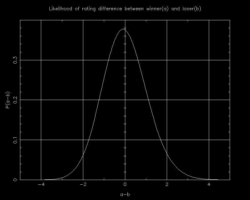
One can integrate over S to calculate P(D). I show that plot below:

While the math is indisputable, this doesn't answer the question of why this is true. To explore that, I present another plot showing P(a,b) as a function of a (on the x axis) and b (on the y axis).

First off, let's verify what should be a common-sense feature: the most likely scenario (i.e. where P(a,b) is maximized) comes where a and b are zero (as is c). This should be the case since the set of games is symmetric and thus this is the only plausible place where such a maximum could conceivably happen. Likewise, although it isn't as obvious from the plot, the expectation value of a-b (the probability-weighted average) is zero, which again is necessary since the average case must be that all three teams have the same rating.
Now for the details. Where a is greater than b, we find that the probability distribution becomes very narrow, meaning that c (which equals -(a+b)) is very tightly constrained. This happens because of the shape of the error function CP(x): the probability is maximized when c is midway between a and b in this case, since having c much lower than a would make A's loss to C extremely unlikely, or likewise having c much higher than b would make C's loss to B extremely unlikely.
However, when A is worse than B, we are in a different scenario. In this case, A's loss to B allows the overall probability to be pretty good whenever c is anywhere between a and b, and thus you see a much broader probability distribution in the upper-left part of the figure.
As it turns out, the amount of probability above the diagonal line exceeds that below it, and thus we conclude that team B is more likely the better team (the odds are 51.2% that B is better) despite its loss to A. This is consistent with the expectation value of a-b being zero because a-b is more likely to be very high if positive, as shown on the plot by the fact that the lower-right extension goes further from the diagonal line than does the upper-left extension.
OK, now let's step back a minute and think about what this implies. Obviously I'm not saying that B is better than A, C is better than B, and A is better than C, since that would be ludicrous. The key to this dilemma is that it isn't a two-team problem, but is rather a 3-team problem. The odds of the ranking order being ABC is 15.4%, which equals the odds of the order being BCA or CAB. In contrast, the odds of having the order being CBA, ACB, or BAC is 17.9%. So the important point isn't really specifically whether A or B is the better team; it is that it is more likely that this 3-way tie was created by the better team winning only one of the three than by the better team winning three of the three. The reason for this is that two minor upsets are less unlikely than one major upset.
For a somewhat more complex (and meaningful) test, I have run the identical tests for a 4-team case in which teams A and B went 2-1, while C and D went 1-2. The sequence of games was A beats B, A beats C, B beats C, B beats D, C beats D, and D beats A. As with before, the question is whether A is likely better or worse than B. The same plots for the 3-team case are shown for this 4-team case. What is interesting about this example is that the 4-team case is very much like the case that comes up: two teams played a variety of inferior teams; the one that beat all of the inferior teams lost to the team that lost to one of the inferior teams.
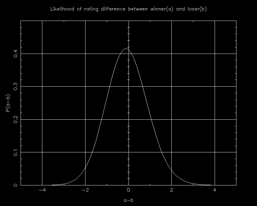
An interesting aside. Using exactly the same calculations for the 1-2 teams, we find that team D is probably better than team C. This means that the most likely scenario is that B is the best team, followed by A, D, and C. In short, the better teams won only 3 of the 6 games in this case, showing again three minor upsets are less bad than one major upset. (Ranking the teams in order ABCD would have only implied one upset.)

This is the last test I will show; you will have to take my word for the fact that this is representative of most cases in which there is a question between two head-to-head teams. (If team A had beaten all of its opponents while team B went 2-1, the whole discussion would be moot since A would be by far the best team. So I'm only looking at situations in which the teams had the same record against an equally-difficult schedule.)
There are several ways to phrase the main conclusions from this:
Note: if you use any of the facts, equations, or mathematical principles introduced here, you must give me credit.